3.2. 如何消除Vuvuzela?

什么是Vuvuzela? 看过南非世界杯的同学们, 肯定会对比赛中响彻全场的Vuvuzela(俗称南非大喇叭)有非常深刻的印象. 本来作为一种庆祝乐器, 但是当这种声音充斥这整个比赛过程, 让听众无法听清到现场解说员的讲解, 大大降低了观赛的舒适度.

那么如何利用数字信号处理的方法将Vuvuzela的噪声从信号中滤除掉呢? 下面我们将介绍一种简单的算法, 来完成这个任务.

Vuvuzela cancellation with spectral subtraction technique. Based on the spectrum of the vuvuzela only sound, this denoising technique simply computes an antenuation map in the time-frequency domain. Then, the audio signal is obtained by computing the inverse STFT. See [1] or [2] for more detail about the algorithm.

References:

[1] Steven F. Boll, “Suppression of Acoustic Noise in Speech Using Spectral Subtraction”, IEEE Transactions on Signal Processing, 27(2),pp 113-120, 1979

[2] Y. Ephraim and D. Malah, ?Speech enhancement using a minimum mean square error short-time spectral amplitude estimator,? IEEE. Transactions in Acoust., Speech, Signal Process., vol. 32, no. 6, pp. 1109?1121, Dec. 1984.

Note: The file: Vuvuzela.wav must be located in the folder of this script file. One can note that this time-frequency based technique creates a “musical noise”.

import numpy as np
import numpy.matlib
import matplotlib.pyplot as plt
from scipy.io import wavfile
import matplotlib.cm as cm
from scipy import signal
from scipy.fftpack import fft,ifft
import sounddevice as sd

print('--- Vuvuzela Cancelation Program ---\n\n');

# load vuvuzela sound example
print('-> Step 1/5: Load vuvuzela.wav:')
Fe, y = wavfile.read('Vuvuzela.wav')
x     = y[100000:].astype('float')
Nx    = x.size
print(' OK\n')

plt.plot(np.arange(0,len(x))/Fe,x)
plt.xlabel('Time (s)')
plt.title('Original Signal with Vuvuzela')
plt.show()

--- Vuvuzela Cancelation Program ---


-> Step 1/5: Load vuvuzela.wav:
 OK

<Figure size 640x480 with 1 Axes>

利用短时傅里叶变换计算语音信号的频谱

短时傅里叶变换(STFT)通常被用来分析非平稳信号的频率成分随时间变化的性质.

对信号进行滑动窗分析, 首先定义长度为\(M\)的滑动分析窗\(g[n]\), 计算加窗之后的信号. 然后,对每个加窗之后的信号进行傅里叶变换:

\[X_{m}(f)=\sum_{n=-\infty}^{\infty} x(n) g(n-m R) e^{-j 2 \pi f n}\]

其中\(R\)为窗口滑动的步长, 且\(R=M-L\). \(L\)为连续两个滑动窗口交叠区域的长度.

# %STFT parameters
NFFT          =1024                               # DFT变换的长度
window_length =(np.round(0.031*Fe)).astype('int') # 滑动窗口的长度
window        = signal.hamming(window_length)     # 滑动窗口
overlap       = np.floor(0.45*window_length)      # 交叠区域长度
#construct spectrogram
F, T, S       = signal.spectrogram(x+1j*1e-16,Fe, window=window,noverlap=window_length-overlap,nfft=NFFT)
# put a short imaginary part to obtain two-sided spectrogram
Nf,Nw         = S.shape

t_epsilon = 1e-2
S_one_sided=np.abs(S[:np.array(len(F)/2).astype('int'),...])
S_one_sided[S_one_sided<t_epsilon]=t_epsilon
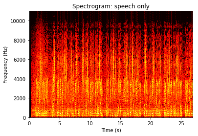
plt.pcolormesh(T,F[:np.array(len(F)/2).astype('int')],np.log(S_one_sided),cmap=plt.cm.hot)
plt.title('Spectrogram: speech only');
plt.xlabel('Time (s)');
plt.ylabel('Frequency (Hz)');

/Users/lyu/anaconda3/lib/python3.6/site-packages/scipy/signal/spectral.py:1819: UserWarning: Input data is complex, switching to return_onesided=False
  warnings.warn('Input data is complex, switching to '

# %----------------------------%
# %        noisy spectrum      %
# %          extraction        %
# %----------------------------%
# Signal parameters
t_min       = 0.4    #interval for learning the noise
t_max       = 1.00   #spectrum (in second)
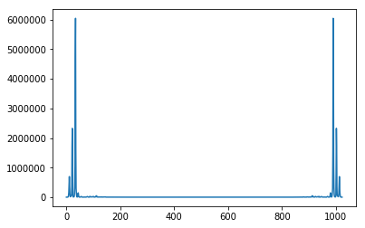
print('-> Step 2/5: Extract noise spectrum -');
absS_vuvuzela = np.abs(S[...,(np.double(T>t_min) + np.double(T<t_max))>=2])**2
vuvuzela_spectrum = np.mean(absS_vuvuzela,axis=1)
plt.plot(vuvuzela_spectrum)
vuvuzela_specgram = np.transpose(np.matlib.repmat(vuvuzela_spectrum,Nw,1))
print('OK\n')
print(vuvuzela_specgram.shape)

-> Step 2/5: Extract noise spectrum -
OK

(1024, 1935)

# %---------------------------%
# %       Estimate SNR        %
# %---------------------------%

print('-> Step 3/5: Estimate SNR -');
absS=np.abs(S)**2
SNR_est = absS/vuvuzela_specgram - 1
SNR_est[SNR_est<0] = 0

# 这里需要进一步对估计的信噪比做滤波处理
apriori_SNR = 1  # select 0 for aposteriori SNR estimation and 1 for apriori (see [2])
alpha       = 0.05      # only used if apriori_SNR=1
if apriori_SNR==1:
    SNR_est=signal.lfilter([1-alpha],[1,-alpha],SNR_est)  #a priori SNR: see [2]
print(' OK\n');


# 以下是显示噪声频谱
t_epsilon = 1e-2
S_one_sided=np.abs(SNR_est[:np.array(len(F)/2).astype('int'),...])
S_one_sided[S_one_sided<t_epsilon]=t_epsilon
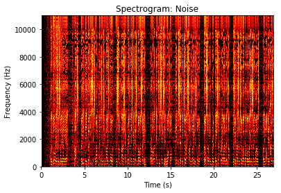
plt.pcolormesh(T,F[:np.array(len(F)/2).astype('int')],np.log(S_one_sided),cmap=plt.cm.hot)
plt.title('Spectrogram: Noise');
plt.xlabel('Time (s)');
plt.ylabel('Frequency (Hz)');

-> Step 3/5: Estimate SNR -
 OK

利用信噪比信息去除噪声

首先定义

\[A_m(f) = \left(1- \frac{\lambda}{\mbox{SNR}_m(f)^{\beta_1}}\right)^{\beta_2}\]

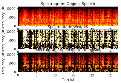
根据信噪比计算每个频谱分量的权重

\[\begin{split}w_m(f) = \begin{cases} A_m(f) & \mbox{ if } A_m(f) \geq 0 \\ 0 & \mbox{else} \end{cases}\end{split}\]

然后利用频谱权重对带噪声信号原始频谱进行加权

\[\hat{X}_m(f) = A_m(f)\cdot X_m(f)\]

原理分析: 信噪比SNR越大,那么权重系数就越大(接近1), 所以加权之后的频谱会保留; 相反, 如果信噪比SNR越小, 那么权重系数越小(接近0), 所以加权之后的频谱就会作为噪声滤除.

# %---------------------------%
# %  Compute attenuation map  %
# %---------------------------%
print('-> Step 4/5: Compute TF attenuation map -');
beta1       = 0.5
beta2       = 1
lam         = 3
an_lk = (1-lam*((1/(SNR_est+1))**beta1))**beta2
an_lk[an_lk<0] = 0
STFT=an_lk*S
print(' OK\n')

# 以下是显示噪声压制前后的频谱
t_epsilon = 1e-2
plt.subplot(311)
S_one_sided=np.abs(S[:np.array(len(F)/2).astype('int'),...])
S_one_sided[S_one_sided<t_epsilon]=t_epsilon
plt.pcolormesh(T,F[:np.array(len(F)/2).astype('int')],np.log(S_one_sided),cmap=plt.cm.hot)
plt.title('Spectrogram: Original Speech');
plt.xlabel('Time (s)');
plt.ylabel('Frequency (Hz)');

plt.subplot(312)
S_one_sided=np.abs(an_lk[:np.array(len(F)/2).astype('int'),...])
S_one_sided[S_one_sided<t_epsilon]=t_epsilon
plt.pcolormesh(T,F[:np.array(len(F)/2).astype('int')],np.log(S_one_sided),cmap=plt.cm.hot)
plt.title('Spectrogram: Weights');
plt.xlabel('Time (s)');
plt.ylabel('Frequency (Hz)');

plt.subplot(313)
S_one_sided=np.abs(STFT[:np.array(len(F)/2).astype('int'),...])
S_one_sided[S_one_sided<t_epsilon]=t_epsilon
plt.pcolormesh(T,F[:np.array(len(F)/2).astype('int')],np.log(S_one_sided),cmap=plt.cm.hot)
plt.title('Spectrogram: Speech after denoising');
plt.xlabel('Time (s)');
plt.ylabel('Frequency (Hz)');

-> Step 4/5: Compute TF attenuation map -
 OK

利用傅里叶逆变换得到时域语音信号

逆短时傅里叶变换通过IFFT计算每一个滑动窗口的时域信号, 然后重叠相加得到时域信号:

\[\begin{split}\begin{aligned}_{x(n)} &=\int_{-1 / 2}^{1 / 2} \sum_{m=-\infty}^{\infty} X_{m}(f) e^{j 2 \pi f n} d f \\ &=\sum_{m=-\infty}^{\infty} \int_{-1 / 2}^{1 / 2} X_{m}(f) e^{j 2 \pi f n} d f \\ &=\sum_{m=-\infty}^{\infty} x_{m}(n) \end{aligned}\end{split}\]

# %--------------------------%
# %   Compute Inverse STFT   %
# %--------------------------%

print('-> Step 5/5: Compute Inverse STFT:')
ind=np.mod(np.arange(0,window_length),Nf)
output_signal=np.zeros([np.int((Nw)*overlap+window_length),])

for indice in range(Nw): #Overlapp add technique
#     print(indice)
    left_index=((indice)*overlap)
    index=(left_index+np.arange(0,window_length)).astype('int64')
    temp_ifft=np.real(ifft(STFT[...,indice],NFFT))
    output_signal[index]= output_signal[index]+temp_ifft[ind]*window
print(' OK\n')

-> Step 5/5: Compute Inverse STFT:
 OK

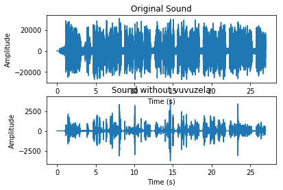
# 显示处理前后的波形
plt.subplot(212)
# plt.plot(x)
plt.plot(np.arange(0,len(output_signal))/Fe,output_signal)
plt.xlabel('Time (s)')
plt.ylabel('Amplitude')
plt.title('Sound without vuvuzela');
plt.subplot(211)
# plt.plot(x)
plt.plot(np.arange(0,len(x))/Fe,x)
plt.xlabel('Time (s)')
plt.ylabel('Amplitude')
plt.title('Original Sound')

Text(0.5, 1.0, 'Original Sound')

# %-----------------    Listen results   ------------------------------------
print('\nPlay 5 seconds of the Original Sound:')
sd.play(x, Fe)
print(' OK\n')

Play 5 seconds of the Original Sound:
 OK

print('Play 5 seconds of the new Sound: ')
sd.play(output_signal, Fe)
print('OK\n')

Play 5 seconds of the new Sound:
OK